2014-02-01T08:00:00+08:00 | Page 2 of 2

Pivot Tables are great in summarizing data from thousands of rows in just seconds. You can get Sum, Count, Average of numbers from any grouping in a Pivot table.

But the one thing that you need at times is a running total in a column. For example, in January, you sold 100 cans, and in February you sold 120 cans. So the total cans you sold till Feb is 100+120=220. This is a running total up to the month of February.

If you want Excel to do this, you can write a formula in the data cells. But to get this thing done in a Pivot Table, you need to use a different way. And it is already pre-built in Excel Pivot Tables, starting from Microsoft Excel 1995.

All you need to do is to click on the Data Field in the Pivot Table Field List, and a popup comes up.

Choose the last option – Value Field Settings.

Move to the Second Tab – Show Values As.

Then select “Running Total in” in the drop-down. Select a base field. It must be a text field, like Product, Category, Region etc.

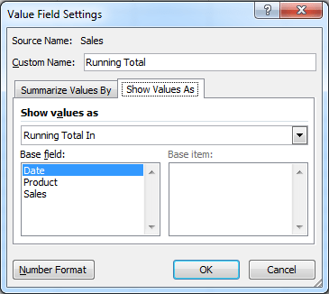
Show Values As - Running Total In — Show Values As – Running Total In

Voila, you get a running total in the data field inside the pivot table. And all you did was to select the correct option. No formulas to write… no calculations to make or check. Isn’t it wonderful?

Using % Running Total In

Similarly, if you choose % Running Total In as the calculation, the running total numbers would be displayed as a percentage of the total. Giving you a much nicer perspective.

Running total Percentage in Excel Pivot — Percentage of Running total

If you’d like to learn more Excel Pivot Table Tricks, here are some additional articles:

Questions About Pivot Tables in Excel?

If you have any questions regarding Pivot Tables in Excel, simply post a comment below and I’ll help you with it. All the best!

And Subscribe to our Excel Tips Newsletter, so we can send you more such Pivot Table Techniques by email. Only useful stuff, without the hype. And we won’t spam you. So don’t worry. Just subscribe.

Cheers,
Vinai Prakash
Founder of ExcelChamp.Net

Vinai conducts 1-2 day seminars and Training Sessions on Microsoft Excel all over the world, helping companies maximize their productivity in using Microsoft Excel. If you would like to find out more, simply contact us.

Are you facing any problem in using Excel? Any Question?

You have come to the right place. Tell us your needs. We’ll be glad to help you!

As soon as you begin working with a larger set of data, this problem of having duplicate values begins to creep in.

And it is most difficult to pick up duplicates. You can use this technique to identify duplicates in Excel. The duplicate values will be highlighted in yellow.

data with duplicates — Data Showing Duplicate Values

But you may not only want to find the duplicates… you actually want to eliminate them completely. In this case, read on, and find how to remove the duplicate values.

First Method: How to Remove Duplicate Cells in Excel

In Excel 2003 and previous versions of Excel, it was extremely frustrating to delete duplicates. You had to write a complex formula, to identify the duplicates first, and then delete them manually or through a macro or a series of steps.

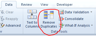
Starting from Microsoft Excel 2007, and continuing in Excel 2010 & Excel 2013, there is a dedicated button on the Data tab, called Remove Duplicates.

All you need to do is to highlight the row of cells which contain the duplicates, and click on the Remove Duplicates button on the Data tab.

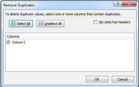
Excel will popup a window to ask about the column, and whether headers exist.

Once you click OK, the duplicates are removed, and you are shown another popup informing you of the duplicates removed, and the number of unique values remaining.

The Resulting data set only has unique values.

Data without Duplicates. only unique values remain — Data without Duplicates.

Do keep in mind that when a duplicate values is found, the first occurrence is considered original, and the second instance is removed. Any other occurrences are also removed. Only the first unique value would remain.

This is a quick and simple way to remove duplicates in Excel.

Second Method: Convert Data Range into a Data Table

If you convert your data into a table, you can use a lot of in-built functionality that only emerged in Excel 2007 onwards.

You can press Control + T to convert a data set into a Table.

Once the data is converted into a Table, you will see a new Tab called Table Tools appear in the Menu bar, at the end of the menu set.

Click on it, to activate the Table Tools Menu.

With the table tools menu, you have another option to Remove Duplicates, which works pretty much the same way as the first method.

The great thing is that the entire duplicate data set is removed completely. The remaining data moves up, and you don’t end up with any blank rows. Thus, no cleanup is required after the duplicate removal.

With these methods, you can remove duplicates, and you can have a clean set of data to perform further data analysis.

Let me know if you use any other methods to identify or remove duplicates.

Are you facing any problem in using Excel? Any Question?

You have come to the right place. Tell us your needs. We’ll be glad to help you!

Additional Resources:

Cheers,
Vinai Prakash
Founder of ExcelChamp.Net

How To Get Running Totals In a Pivot Table

Are you facing any problem in using Excel? Any Question?

Removing Duplicate Values in Excel

Are you facing any problem in using Excel? Any Question?

Get Excel Tips & Tricks Each Week

Get Excel Tips & Tricks Each Week