Multiple Ways to Count in Excel

Counting the number of cells containing values, counting number of cells meeting a certain criteria, counting names, counting cells in a range…. you name it, there is a need to count in Excel. And there are multiple ways to count in Excel. Some techniques are more helpful than others, and some can provide unique insights which others can’t produce.

Let’s look at the different ways to count in Excel, and their relative benefits.

1. Count the number of cells with values: The simplest way is to use the inbuilt function Count. Select the cell range, and out comes the cou nt of cells in the range.

Count only works with counting of Numeric information. If you try to count names, you will get a ZERO.

To count alphanumeric values – values with names, categories, text, serial numbers etc., then you must use the variation of Count – called COUNTA. This function is to count Alphanumeric data.

Count of Numbers in a Range, & Count of Names in a Range

2. Using a Criteria to Count specific Cells: There are several ways to count the cells that meet a certain criteria. The first method treats the data as a database, and uses the Database Functions within Excel.

=DCOUNT(Database, Field, Criteria)

Count the cells that meet a specific criteria using Dcount

Here A4:C12 is the entire data, B4 is the cell column that we want to count, and the criteria is Age should be greater than 30 years (B1:B2) cells.

The answer for this count is 5. See if you got this correct.

The database functions have been existing in Excel since 1995. They treated Excel data as a database like Oracle, Dbase etc. These database functions DSUM, DCOUNT, DAVERAGE etc. are quite useful, and are available for backward compatibility, although the same work can be accomplished by other functions equally well too.

3. Using COUNTIF Function to count cell conditionally. This method evaluates the cells against the condition, and if it matches, it is counted.

=COUNTIF(Cells, criteria)

Count cells that match a condition

Here, the cells that contain the data is provided first, and the second argument is the criteria. The headings are not really needed. Each cell in the first range is checked against the criteria, and if the criteria matches, the record is counted, otherwise it is ignored.

Want to Improve Your Excel Skills?

Learn the Key Features of Excel Quickly & Easily, by Joining the
Online Training on Basic / Intermediate Excel.

To Get Most out of Excel, Learn theĀ  Pivot Table techniques in our
Pivot Table Masterclass Training
!

And if you have multiple criteria to check for, you can use the COUNTIFS which can take multiple criteria arguments.
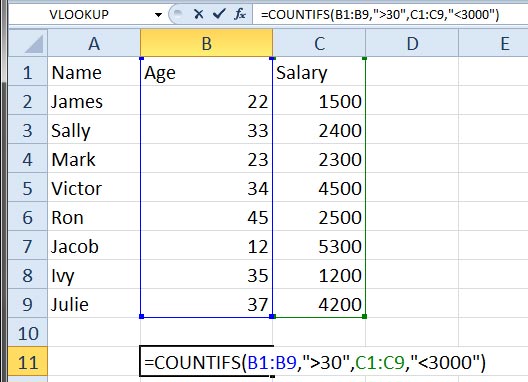
CountIFS to count cells with multiple criteria cells.

The formula in the picture captures the count of cells that are having age of >30years, and Salary less than $3000. Answer is 3.

So as you can see, there are multiple functions, and ways to count cells in Excel. It depends on whether you want to count numbers or textual data. It also depends if you have conditions or not.

Use these functions to count in multiple ways… Happy counting!

Cheers
Vinai Prakash
Are you facing any problem in using Excel? Any Question?

You have come to the right place. Tell us your needs. We’ll be glad to help you!

Additional Resources for Learning Excel & Become A Pro

  1. Top 12 Most Important Excel Functions You Absolutely Must Know
  2. Excel Beginners Guide
  3. Excel Essentials: From Beginner To Pro in Just 6 Weeks

Creating Beautiful Excel Charts For Business Presentations

Microsoft Excel is used to produce charts that are used in the boardroom, in business presentation, and in school projects all over the world. However, most people do not go beyond the standard charts that Excel produces by default, which could be the most boring, and most unsuitable of charts.

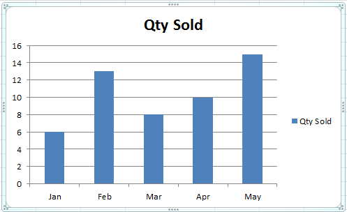
In this article, I am going to show you how you can add value to the default Excel chart, and make it really sing, with just a few clicks. Plus a few tips on how to put some glamor, some jazz, some oomph to your charts to make them beautiful, sexy and cool!Excel Default Chart... Not the most exciting chart.

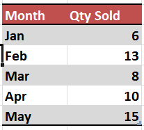
Remove Chart Junk: The default Excel chart has a lot of junk. See the before and after picture below.excel_chart_data

Now let’s see how to arrive at this result ourselves. If you would like to try it yourself, see the image above for the Excel data file with the original data showing. You can key in this data to get started yourself.

improved_excel_chart

Want to Improve Your Excel Skills?

Learn the Key Features of Excel Quickly & Easily, by Joining the
Online Training on Basic / Intermediate Excel.

To Get Most out of Excel, Learn theĀ  Pivot Table techniques in our
Pivot Table Masterclass Training
!


1. Move Legend to the Bottom: The default Legend on the right side of the chart steals away valuable space from the chart. So move it to the bottom. Simply Go to Chart Layout Settings, and Click Legend, then select Bottom. The legend moves to the bottom, and the chart bars now have more space to expand.

2. Remove Grid Lines: Sometimes the grid lines do not add much value, and are best eliminated, as they just make the graph look cluttered.

3. Show Data Values: You can show data values on top of the bars, inside the bars, or at the bottom. Once you have the data bars showing, you really do not need the grid lines anyway.

4. Remove the Vertical Axis: If the values of the data bars, and the Title of the chart are self explanatory, then you can get rid of the vertical axis, giving you more room.

5. Add a Chart Title, Above the Chart: Choose the Title from the Layout, and then select “Above Chart”. This way, your data will never hit the title.

6. Change the Theme: Most people live the default Office theme. But Excel provides over 50 different themes, which can make your charts look much sharper, out of the box.

7. Apply Custom Colours: If the theme colours do not suit you, you can pick any colour you like for any data bar or pie.

8. Add a Company Logo: You can add an image anywhere in the chart. It could be your company logo, or any particular product. Do not add clipart for the sake of adding it. It looks quite cheap and amateurish.

With these simple tips, you can improve your charts and graphs, and give them a new lease of life… make ’em jazzy, snappy, and cool!

Cheers,
Vinai Prakash

Are you facing any problem in using Excel? Any Question?

You have come to the right place. Tell us your needs. We’ll be glad to help you!