Excel Functions | Page 2 of 5

How To Summarize Data in Excel: Top 10 Ways

December 3, 2023September 3, 2021 by Vinai Prakash

You’ve got some data in Excel, and you want to summarize it quickly. There’s not much time, and your client or boss needs information right away.

Apply any of these Top 10 Techniques to Summarize Data Quickly with in-built Excel Functions and Features. You’ll get instant results to satisfy most requirements fast.

Microsoft Excel has become the easiest way to analyze data quickly. Several Summary functions, Pivot Tables, What-If Analysis, and other powerful features & methods are available for your use within Microsoft Excel right out of the box. Learn them, and your data analysis will become a breeze.

Here are the Top 10 Ways to Summarize Data in Excel Quickly

These data analysis & summarization tips will work in Microsoft Excel 365, Excel 2019, Excel 2016, Excel 2013, Excel 2010, Excel 2007 & even Excel 2003. Further, they work on Excel for Windows as well as Microsoft Excel running on a Mac.

These Data Summarization Tips are listed in the order of the easiest to implement to the ones that need a bit more time. Some of the more complex data summarization methods will actually add more value to your data analysis.

Get The Data Ready For Summarization
Quick Summary With Auto Functions
Fast Analysis With Sort & Filter
Summarize Data With SubTotal Feature
Summarize Data With an Excel Table
Using Slicers to Summarize by different dimensions
Summarize With Excel Pivot Tables
Summarize Data With Excel Functions
Advanced Excel Functions for Summarizing Data
Summarize With Descriptive Statistics From Analysis Toolpak

You can apply the different ways to summarize data based on your familiarity with Excel.

The easiest methods of summarization are listed in the beginning.

And the Pivot Table technique is one of my favorite for a quick and dirty data summarization within Microsoft Excel. It always begins to give me numerous insights into the data.

We cover how to use the Pivot Table to Summarize Data in depth later in this article.

Let’s get started by exploring the different methods of summarizing data.

1. Get The Data Ready For Summarization

Before you begin your summarization, it is important to make sure that your original data is in a good shape.

Duplicate, a blank cell or missing values can often spoil your data summarization.

You need to make sure that the data range is correctly set up before you begin to analyze the data. Also, ensure there is no blank columns in between adjacent cells.

Ensure Proper Column Headings.

For each column, make sure that you have a short and unique column heading. Don’t leave any column without a heading, even though it may be obvious. Column Heading will make it easy to analyze data with any tool in Excel. This way the top row becomes the Header row.

Remove any Duplicates.

Duplicate rows can often sneak in from the data capture sources. So whether you capture data from the Web, or SalesForce, SAP or load from Text or CSV files, the first thing is to clean up the duplicates. To remove duplicates, click within the data range, and go to the Data Menu.

Data > Remove Duplicates.

That’s it, your data will now be cleaner.

Get Rid of Blank Rows:

While blank rows make the data look more readable and easier, it is a bane for data analysis. We do not want blanks to sneak in and skew our averages and other statistical calculations. By sorting the data with the different column headings, the blanks will get separated either to the top or to the bottom. Then you can simply delete these rows if they do not contain any other data points.

Don’t leave blank cells as blanks, specially if there is no value.

It is better to have a 0 than a blank value in any cell. For the text column, if the value is not known, it is better to have a NA (Not Available) showing up.

Having the data cleaned up is the first step in any data analysis. Now you can begin to apply the various data summarization methods.

2. Quick Summary With Auto Functions

The fastest way to summarize data is to calculate the Totals, count the number of entries, find out the average value, and figure out the highest and lowest values.

These 5 functions provide the vital stats of the data. These are the most basic and essential functions… just like a visit to a doctor starts with the nurse checking your vitals – height, weight and blood pressure.

These 5 numbers will provide a quick summary of your data. Here’s how to do this.

Here’s How To Create a Summary Section on Top of Your Data

Calculate SUM: Click on the Autosum icon on the Home tab of Microsoft Office to activate the Sum function of Excel. Then select the data range of the column you want to summarize. Here’s an example:

Calculate COUNT: Click on the drop-down icon on the Autosum button on the Home tab of Microsoft Excel. Choose Count from the list. Then select the data range of the column you want to count. You can use the count function only for numeric columns like Salary, Sales, Quantity etc. using this function. So don’t try this on a text column like Country or Department.

Calculate AVERAGE: Click on the drop-down icon on the Autosum button on the Home tab of Microsoft Excel. Choose Average from the list. Then select the data range of the column you want to Average. You can only average the numeric columns like Quantity, Profit, ROI etc. using this function. Here’s an example:

Calculate Highest Values: Click on the drop-down icon on the Autosum button on the Home tab of Microsoft Excel. Choose Maximum from the list. Then select the data range of the column you want to choose for picking up the highest value. You can only pick numeric columns like Quantity, Profit, ROI etc. using this function. Here’s an example:

Calculate Lowest Values: Click on the drop-down icon on the Autosum button on the Home tab of Microsoft Excel. Choose Minimum from the list. Then select the data range of the column you want to choose for picking up the lowest value. You can only pick numeric columns like Quantity, Profit, ROI etc. using this function.

Calculating the Sum, Count, Average, Min & Max are the fastest ways to get started in your journey to view summary data quickly.

3. Fast Analysis With Sort & Filter

If you sort the data by any key column like Country, Department, Category, Product, Zone, Area etc., then it becomes super easy to analyze data.

To sort the data on any column, follow these steps. Go to

Home > Sort & Filter > Sort A to Z or Sort Z to A.

This will sort the data in your chosen way (ascending or descending) for the column you are in.

Then click on the Filter icon. This will set up auto filters on top of all column headings. Now when you filter on any column, only values for that column will be visible. Unfiltered values are hidden, and visible data corresponds to the Filter selections.

After you have filtered for any particular selection, you can also highlight any numeric column, and see the summary being displayed at the bottom Excel bar.

At one time, you can see the Sum, Count, Average, Maximum & Minimum values from the selected range.

Now you can begin to summarize data for any selection, the way you want it.

4. Summarize Data With Subtotal Command:

If the data is already sorted, you are now ready to explore the Subtotal feature of Excel. This hidden gem has been languishing in Excel since the early 1990s, and very few people use it.

To add subtotals to your summary, first, clear all filters. And then Sort on the column that you want to add subtotal for.

The Subtotal feature is available on the Data tab of Excel.

Go to Data > Subtotal.

Choose the function to perform (Sum, Count, average etc), for the numeric column, and group by the desired column.

As an example, to get the subtotals of the number of employees by each department, it should say: At each change in Department, Count, number of Employees.

Using Subtotal to Summarize Data in Excel

Click OK, and you should see the subtotal rows from the data in Excel. In the end, you will also see the Grand Totals calculated.

Result of Subtotal Command in Excel — Results of Performing a Subtotal in Excel

You can clear the subtotals, and perform the subtotals again at any time. To clear the subtotals, go to Data > Subtotal > Remove All. The subtotals and the Grand total row are all removed completely.

5. Summarize Data With an Excel Table

Microsoft Excel 2007 brought a new feature called Tables, which are amazing at doing simple summarization from a table of data.

To begin, stay within the data range on the Excel sheet. Then click

Home > Format as Table.

Select any colour you prefer, and click OK. Excel automatically recognizes whether the data selection has headers or not.

Now you have a new tab added to the Excel menu, at the end. It is called Table Design.

Select it, and check the Total Row checkbox. Now you have an additional total row added at the bottom of the data. Every column on the total row is a total calculator. Simply click on the dropdown showing in the total row cells, and choose an appropriate summarization – sum, count or average. Now that column will show a total sum or total count or total average of that column.

The great thing is that now if you filter the list, the totals will change dynamically. No need to call the Subtotal function every time. This technique of data summarization is better than the manual methods of subtotal.

Result of Table Counts in Excel — Results of Total Row in an Excel Table

Begin using the Table features if you haven’t done so already.

6. Using Slicers to Summarize by different dimensions

Beginning Excel 2010, Microsoft added the Slicers functionality which takes the Tables to greater heights.

Instead of filtering each column one by one, you can now create a slice of the data from the Excel spreadsheet at any time.

Go to Table Design > Insert Slicer > Pick the column of your choice that you want to filter on.

Now you can click on any value in the slicer, and the data is instantly filtered. You can make multiple selections, by holding the control key.

And more than 1 slicer can be added, giving you multiple combinations of slices. The total row updates automatically as each selection is made. This is truly slice and dice of data, allowing you to summarize data in Excel spreadsheets just by using a mouse. No formulas or lengthy steps are involved.

7. Summarize With Excel Pivot Tables

Pivot tables have been in Excel for over 30 years. They are the most used feature of Excel, as it allows for business analysts & managers to manipulate and analyze data in countless better ways.

A pivot table is actually a summary table, which allows you to slice and dice the data by different dimensions.

Pivot tables are easy to get started with.

To create a pivot table, Stay within your dataset. Then go to Insert > Pivot Table. The entire dataset is selected. Click OK and a new pivot table is created in a new worksheet by default.

Click on the column that you want to summarize on, from the pivot table field list on the right side of the screen. In our example, we check the Department and Sales amount from the field list. Instantly, the total sales per department are calculated and populated in the pivot table on the left. Notice that Excel generates a unique list of departments, without any duplicates.

To visualize both the Sum & Count of the data points, you can drag one more copy of the Sales into the Values Area section. Then right-click on the value, and choose

Summarize Values by > Count.

Similarly, you can change the calculation type, and pick up Average, Max, Min. This way, you can have all the vital statistics about your data summarized by each department.

Additionally, to see the percentage of sales done by each department,

Right Click on any numeric value in the pivot table, and choose Show Value As > % of Grand Total.

This will instantly calculate the % of contribution done by each department. The grand total will show 100% of the sales.

It is a good idea to sort the % of Grand Total value from highest to lowest by value, showing the highest values on the top.

You can then add a further selection in the rows or columns, to get a 3D view of your data. As you can see, Pivot Table is a powerful tool that can get the analysis done the fastest!

As you learn more about the Pivot Tables, you’ll realize that they can be used to summarize data from a single worksheet or multiple worksheets.

A pivot can even summarize data from multiple workbooks too. This is a must-learn feature of Microsoft Excel. You can attend an Advanced Excel Training in Singapore at Intellisoft, where I teach this class.

FREE COURSE ON PIVOT TABLES TO ANALYZE DATA – No Signup is required. Click & Start watching Videos For Free and improve your Pivot Table Skills.

8. Summarize Data With Excel Functions

To get the most flexibility, you can actually write your own summary functions within Excel, by using the following formulas.

We have already covered the Autosum features of Excel which generate the Sum, Count & Average. Now we will look at how to write these functions manually.

To Sum a range of data, use =SUM(range) in the formula bar.

To Count a range of numeric data cells, use =COUNT(range). This generates a numeric count.

To count a range of alpha-numeric data cells, use =COUNTA(range). COUNTA can be used to count both numeric and non-numeric data.

To find the average of any data, use =AVERAGE(range).

9. Advanced Excel Functions for Summarizing Data

The real power of Excel functions is when you go beyond the basic summary functions and do some advanced data analysis.

You can use the following Excel formulas

Sum the data conditionally. For example, if we want to summarize the monthly sales only for a particular country, we can use the Excel Sumif function:

=SUMIF(country data range, select_country, monthly sales data range)

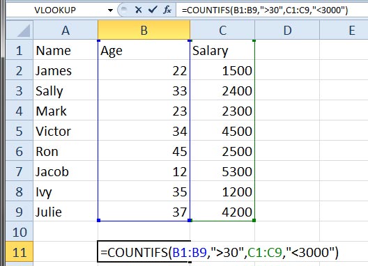
Similarly, to count the number of products sold by a country, we can count by using the COUNTIF function of Excel

=COUNTIF(country data range, select_country, monthly sales data range)

And average sales per country can be analyzed by using the following formula of AVERAGEIF.

=AVERAGEIF(country data range, select_country, monthly sales data range)

For multiple, if conditions, you can use the sumifs function to summarize data by your chosen selection. These functions can really cut down your data analysis time when you have large amounts of data to summarize.

10. Summarize With Descriptive Statistics From Analysis Toolpack

Finally, Microsoft Excel has the Data Analysis Toolpak, a hidden Statistical Analysis tool, that can calculate the Median, Standard Deviation, Variance, Analysis of variance (ANOVA), and much more in a single click.

To enable the Data Analysis feature in Excel, you must go to

File > Options > Add Ins.

Then select the Data Analysis ToolPak if it is inactive. You might have to click on the Go button at the bottom. Choose the Toolpak, and click OK. This will add a Data Analysis button on the Data tab of Excel, at the end. Check it out. Once this button is enabled, it stays active, and you can use it subsequently anytime.

To use this Data Analysis ToolPak, go to

Data Analysis > Descriptive Statistics.

Select the Entire numeric column that you want to analyze in the Input Range. Check the Labels in First Row checkbox if your data has a header.

Then check the output box radio button, and key in a cell address where you want the summary statistics to be generated. Check Summary Statistics, and click OK.

The full descriptive statistics are displayed instantly. This final result is a detailed Statistical Analysis of your data.

Descriptive Statistics Result from Analysis Toolpak

Multiple Ways to Summarize Data in Excel – Conclusion

There are so many different ways to summarize data in Excel. Mastering them will improve your data analysis skills, and you will be on your way to huge success, by taking action on the insights gleaned from your data analysis.

Go ahead and try them out.

Each technique is a gem, and adds to your skills in Excel data analysis.

Cheers,
Vinai Prakash

About Vinai Prakash: Vinai is a prolific speaker, author, entrepreneur and coach on the topics of Data Analytics, Project Management, Advanced Excel Techniques, SQL, Python, Data Visualization with Power BI & Creating of Excel Dashboard and several other soft skills. He is one of the Best Trainers for Data Analytics Training and is highly sought after for his advice. Contact Vinai for your next Data Analysis Training.

Join Vinai’s Data Analysis With Excel MasterClass, and learn how to analyze data firsthand.

How To Learn Advanced Excel Fast

December 3, 2023August 16, 2021 by Vinai Prakash

Advanced Excel skills are required in most managerial & analyst roles. Yet most people have no clue of how to learn Advanced Excel fast. They don’t know the key features of Microsoft Excel that can help them save time and money.

It’s about time you pick the Most Important & Useful features of Excel quickly. This post coveres the following topics in detail.

What is Advanced Excel,
Why should you learn it,
How to learn Advanced Excel Fast!

Welcome To This Short Guide to Being an Expert in Advanced Excel Skills

Every organization uses Microsoft Excel in their day to day work. Most employees & managers know Excel to some extent. And they are able to survive the day by doing things in one way or another… often the long and inefficient way.

Learning to use Microsoft Excel well goes beyond the basics. That’s where the Advanced Excel skills come in handy.

Microsoft has bundled in hundreds of useful functions and features, that can do wonders, save a lot of time, and improve your efficiency & productivity.

Each new version of Excel is packed with ever richer functionality, and provides more ways to use Excel to its utmost at any workplace.

Microsoft is striving to add those features that can simplify complex things, and make it easier to do data entry, perform computations, and even analyze data & present the insights into actionable information useful for clients and colleagues or the management in nicely created reports and dashboards.

So how come very few people are familiar with these Advanced Excel Features & Functions?

Partly because Microsoft is a software company, and not so much an education company. They add new Excel formulas, features, shortcuts, buttons, charts types, and options, but Microsoft doesn’t spend the time in educating everyone about these new enhancements in the time they deserve.

Microsoft simply blog about it, updates the documentation, and then wait for you to figure it how somehow. Most greatly useful features languish, forgotten in the documentation, hardly ever used…

Also, partly to blame is our education system, which does not start teaching us the key Excel skills that are essential in the job. Almost every student now works on a laptop or a tablet, using documents & spreadsheets for every report, presentation or assignment they do. But our schools often leave you to figure how to be productive with these basic tools.

Very few schools or colleges have mandatory Excel or Word Training. It’s no wonder that when a fresh graduate joins the workforce, they often take ages to do simple things, stumbling and faltering along their journey to do even basic things in Excel, let alone the Advanced Excel Techniques that are required to be productive.

Why Should I learn Advanced Excel?

That’s a common question for people using Excel at workplace. If you don’t even know what Excel can do, why will you be interested in learning it. You need to see the features to believe it, and to see your own blind spots.

Increased Productivity With Advanced Excel Tips & Tricks

If you care about getting the job done faster, without any errors, then it is in your interest to improve your competence in Excel. You don’t have to learn all the 500 plus functions to master Excel. In fact, you can already be more productive if we can know and use more than 10-15% of the Advanced Excel features and functions we have listed below.

Better Job Prospects With Better Excel Skills

New job prospects & Career switch options also open up for those who can manipulate and juggle data easily in Excel. Many higher end analyst jobs in the financial and accounting, sales, marketing, management & consultancy areas require good analytical & decision making skills.

Better Presentations With Excel Charts, Reports & Dashboards

Plus, With Advanced Excel Charts & Reporting features, you can be a star in the boardroom too. Most client presentations will need some amount of data and analysis to be presented, which can easily be analyzed and tabulated in Microsoft Excel, provided you know how to do it quickly.

So now you know the key reasons why you should learn Advanced Excel, you may be wondering, what are the key features of Excel that can considered as “Advanced“.

What Really Are Advanced Excel Skills?

Knowledge of multiple useful features and functions, plus the ability to use them at short notice is what we can call as Advanced Excel skills. To name a few, you must be able to know and perform the following things in Excel well.

FASTER SETUP & DATA ENTRY WITHIN EXCEL

Setup Columns Quickly using Auto fill options. For example, you can fill Months or Quarters easily by filling in just the first value. Similarly, you can generate sequence numbers from any starting point to any ending number.

Do Quicker Data Entry by using Auto complete of repeating values as Excel picks up the filling values using pattern recognition
Generate Sequence Numbers quickly With Auto Fill & FlashFill options

LOADING EXTERNAL FILES & DATA

You must be able to Bring External data into Excel from any kind of source – be it Text files, CSV files, XML, Web Data or Database files. Plus, Excel now makes it easier to bring in data from the Cloud Apps like SalesForce, Zendesk, QuickBooks & over 200 app integrations, from PowerQuery, now built into Excel, from version 2013 onwards.

All is not good just by loading the data. You will have to clean & de-duplicate it. Fill in blanks, handle null or missing values, and then fix the dates to become useable. You’ve often got to convert dates formatted as YYYYMMDD or DDMMYY into something that’s more humane – DD-MMM-YY or MM/DD/YY. Obviously the actual settings will depend on your country, regional settings & preferences. But it is often required. This requires you to use PowerQuery, or use Text functions to extract the date, month or year from strangely formatted dates.

EASIER DATA FORMATTING

After cleaning the data comes the job of making it easier to read and identify the key data points.
Here comes the Data Formatting options. Formatting Data makes it easier to read and present data. With Conditional formatting options, it is easier to highlight data based on any simple or complex condition or criteria. By highlighting data, you can make it easy to the winners and losers & spot issues and errors. Highlight the highest values, lowest values, values between a range, values outside a range, or set up your own rules, based on calculations.

LEVERAGE ON IN-BUILT EXCEL FUNCTIONS

Good knowledge of Advanced Excel Functions is essential to get more mileage out of Excel. Microsoft’s Excel functions are divided into multiple categories:

Lookup Functions like VLookup, Index, Match, Offset, Indirect allow you to find anything from within Excel tables and Master data. Pick the employees name based on Code, or find out who secured the highest or lowest sales numbers.

Statistical Functions like Median, Mode, Standard Deviation, Variance allow you to analyze data statistically. You can find out the median, standard deviation or variance, allowing you better insights into the data as to what happened, why it happened, and what is most likely going to happen.

Analysis Functions like Correlation & Regression, Trend Analysis & Forecasting further the statistical functions into forecasting, and allowing you to make better projections, and better decisions based on the happening trends.

Logical functions like If, Sumif, Countif, Iferror allow you do things conditionally – check if a condition is met, add or count based on conditions being met or not met, and even check and handle errors from happening.

Date & Time functions for finding todays date, time, difference between dates, hours, year, month, days, weekdays. This allows you to do time based calculations, buckets of date ranges, and even create ageing analysis based on range values.

Database functions that treat the entire data set as a database, and allow you to aggregate results using Dsum, DAverage, Dmax, Dstdev. This can be useful when working with big data

Text Functions to extract, clean and manipulate data – Left, Right, Mid, Char, Len, Fixed, Trim, TextJoin help in fixing erroneous data, and picking certain batch codes, lot numbers, region or product codes from within serial numbers.

Financial Functions like PV, NPV, PMT, IRR, Accrued Interest, Future Value, Mirr etc. are useful for analyzing the current, present and future value of things. Interest calculation, accruals, monthly installments, interest rates etc. can be easily worked out by using these advanced Financial functions of Excel.

PIVOT TABLES FOR QUICK ANALYSIS

Use the Pivot Table feature of Microsoft Excel, which is the fastest way to get some high level summary from your data set. Pivots allow you to slice and dice the data in numerous ways, and analyze it using different dimensions easily, without writing any formulas or macros. A pivot table is the first thing people turn to when they want some quick analysis or summary on the data.

With the help of Slicers, Timelines, Report Filter Pages, you can look at the same data in multiple ways, multiple dimensions, and in multiple filter flavors.

These are all great ways to analyze information quickly with Excel – a strong reason to learn Advanced Pivot Table techniques of Microsoft Excel.

Use Excel Pivot Tables For Quick Analysis

In fact, knowledge of Pivot tables is often tested in interview questions for jobs requiring a good amount of business analytics. Even in days where most companies world class ERP software with hundreds of canned reports, often raw data is extracted from these ERP packages and combined with external market data, manual forecasts and then analyzed using Pivots.

Competence in Advanced Pivot Table analysis techniques are are must if you want to get into business analytics. Strangely, for the amazing things pivots can do, they are surprisingly easy to master. I often see managers and senior executives surprised at the simplicity, and lament that they missed out on this easy feature for the past several years, relying on junior executives to churn out the reports.

No harm in getting the ground staff to run the reports, but sometimes they do not have the acumen or sensory acuity of understanding the big picture. The juniors often report the obvious, without being able to get that helicopter view of the data.

Pivots are the easy, low hanging fruit that you should begin with, for it brings the biggest bang for the buck. You can easily master it in an afternoon, or in a pivot table masterclass and win an edge with this winning Advanced Excel trick up your sleeve.

CHARTS TO VISUALIZE INFORMATION

Create Charts from raw or summarized data to visualize the information quickly. Multiple columns and thousands of rows make it very difficult to see the big picture and spot a trend.

A visual is worth a thousand words. An Excel chart can depict the past sales of many months or quarters, returned products or problem tickets created/solved each month, and it becomes much easier to spot a trend by looking at a high level chart more than by looking at a sea of rows and columns

There are multiple kinds of charts in Excel that can make boring data look stunning. Choose from Bar & Column charts, Pie & Donuts charts, Waterfall charts or Line Charts. You can also create combination charts showing column and lines at the same time, allowing you to measure 2 different metrics at one time.

Excel charts are easy to master, and there’s a lot to choose from. You can easily format them, add legend, titles, colors, and just about tweak every aspect with a mouse click. Mastering such Excel Charting tips can take you far in the boardroom, with better looking charts & visuals.

MACROS IN EXCEL TO RECORD & AUTOMATE STEPS

Macros are the one Advanced Excel Feature that allows you to extend Microsoft’s products and take them to newer heights. You can create your own functions & automations in Excel to perform multiple steps in a short time, at a single button click.

Macros are heavily used in Banks, financial institution, and in accounts departments of almost each and every company. They are the staple of the data enthusiasts who like to do things just once.

Excel VBA Macros allow you to load new data automatically each month, collate and tabulate multiple sheets & multiple workbooks, and create reports & charts automatically for each new period.

Macros are recorded or written and edited in a special language created by Microsoft – Visual Basic for Applications (VBA) in short.

While learning VBA may take some time, this is the secret weapon that separates the wizards of Excel from the amateurs. Once an Excel macro is written and tested, it can easily be deployed to the masses. Your colleagues and users needn’t know the complexities or the logic of how things are done.

For example, you could create your own custom Financial Accounting Software, just by using Excel. Using Forms, you can get the users to key in the sales, expenses, and generate invoices or receipts at a click. And a Cash Flow Statement, a Profit & Loss Statement, or a Balance Sheet could be generated at any time, collating all the data keyed in so far.

This allows the users to get more done with Excel, and everyone doesn’t have to learn the technicalities of generating such reports at any time.

VBA Macro writing and editing skills are considered Advanced, because it requires you to learn the specific way Excel refers objects like workbooks, sheets, rows and columns. VBA is a full blown programming language – allowing you to write loops, conditions, procedures, functions, and tag them to buttons, mouse movements etc.

This one advanced Excel skills can make you indispensable in the whole department. I have known several people who have a clout in the company because of their deep knowledge of the system, and that they have written the backend systems that the company uses in its day to day operations. Such deep knowledge is always in demand.

SHARING & PROTECTION OF DATA

Today Microsoft Excel is improved and enhanced to allow multiple colleagues and friends to work together on the same file. You can track changes of who did what, and you can even protect the information in such a way that only those authorized to see or edit can do so, protecting information from prying eyes.

With Advanced Data Protection techniques in Microsoft Excel, you can hide sheets, write protect them to make them view only, or allow only certain rows, columns or cells to be editable. This gives a tremendous advantage while working with multiple people and multiple sheets.

With the integration of OneDrive, you can truly collaborate with your team, having multiple edits and track changes as they happen. It is much easier to edit, pick the changes you like, or remove/revoke changes that you do not approve of.

If you haven’t visited the Review menu of Excel, you’d be surprised with the multiple options available under the hood, that allow for Collaboration, Sharing, Editing & Protection of Documents.

SIMPLE, COMPLEX, ADVANCED TEMPLATES

Almost everything you do in Excel has been done before. So if you are making a calendar, or a cash flow report, a monthly report, attendance report, Result of Students, Invoices or Statement of accounts, Expense claims or Employee Leave forms for the team, there is a ready made template to do so.

Not just one, you have hundreds of templates to choose from. These ready made templates are available to any Microsoft Office user to use and save time.

On top of this, you can create your own company wide or departmental templates, that can be used month after month, quarter after quarter without any changes. Consolidation becomes a breeze if you all use the same template.

Plus, tracking & merging of multiple changes can be done with the hidden Track & Merge option. You can’t find this button in the standard toolbar, and need to enable it separately. A golden gem of a function. Even seasoned pros have been unaware of this super cool advanced excel functionality.

Print Beautiful Reports & Charts With Advanced Excel Techniques of Page Setup

With Advanced Page setup, you can decide what you want printed and what not. You can add headers, footers, page numbers, logos etc. straight out of the box. But Excel goes beyond this into giving you fine control over the rows, columns, and area that will be printed.

You can control whether you want to print grid lines, draft copy or are you printing the final copy. The current date or time can be printed too, along with a lot of meta data – file names, sheet names, page numbers etc. provide you with a fine control. Printing order – collated or by page, and auto fit to handle orphan printing of some columns can be a real paper saver.

Trees will love you for learning and using the page setup options within Excel well.

ADVANCED SORTING & FILTERING

Almost everyone figures out how to sort data on any column – in either ascending or descending order. But Excel allows you to perform custom formatting – based on your values, and your defined order.
Sorting for multiple, unlimited levels is a boon too. This breaks the limited 3 level sorting of previous versions, allowing you to sort as many levels as you please.

Filters have improved much in the past 10 years. Now you can easily filter the Top 10 or Bottom 10 values, filter by color, filter by values, and even filter by specific text or dates. There filter feature helps you to actually define the period of data or values that you want to focus on, and eliminate the rest. Master this simple feature, and get to your important data points quickly.

Filtering the values to focus on at any given time removes clutter and makes it easy to visualize information in Excel.

FORMATTING DATA INTO TABLES – A SUPER SIMPLE WAY TO ADD MAMMOTH FUNCTIONALITY, For Free!

Microsoft added the functionality to treat data as a table in Excel 2007. But the name they gave to the button that begins this functionality is a showstopper.

When you look at “Format As Table”, all you’ll see is multiple coloured data tables. And many an Excel enthusiasts pull away, thinking its just colors… They fail to learn the mammoth hidden functionality of Excel beneath this mis-labeled button.

But once you go over this hump, you are on your way to explore gold with Formatted Tables.

Since 2007, Excel Tables have come a long way. Now they have smart range names, auto fill and auto spill ranges, and use range names in calculations. There are several magic cells in Excel Tables, that can perform additional tasks too.

Becoming adept at using Table features of Excel will speed up your analysis.

Further, tables can be filtered, sorted, sliced. For date based data, you can add a Timeline, which is a slicer based of dates, but much better.

There you have it… These are just some of the advanced features of Excel. Learning about additional things like Custom Formatting, Range Naming, Working With multiple Worksheets, or combining data from multiple workbooks, consolidation, What-if analysis, Scenario Manager, Data Tables, Data Validation etc. will take your Advanced Excel knowledge to a much higher level. There is simply too much functionality to talk about in one article.

Suffice is to say that if you want to get done more, cheaper & faster, then learn some of these Advanced Excel Features, pronto!

How long does it take to learn excel?

There is no simple answer when you are beginning to learn a new skills. To learn Advanced Excel tricks is going to be the same too. It also depends on your interest, commitment, and the amount of time you are wiling to spend in learning it.

I would say that learning Advanced Excel tips and tricks is more of a journey.

You learn some concept, begin to apply it, and then learn some more. While learning, you will come across new concepts, see new problems, and seek newer ways to handle these challenges. This step by step approach will open your eyes, develop a keener sense of Excel capability, and develop your Excel muscle step by step, day by day!

I have been a student of Microsoft Excel for the past 30 years. And still I find new things, and new ways of doing the same things. It has been a fun and exciting journey and I love challenges in Excel.

Every once in a while, someone will send me a long and complex looking formula, and dissecting it, understanding it, and learning from it makes us all better. Helping others with their Excel has been one good way that has helped me grow my Excel competence.

Can you teach yourself Excel?

Yes, of course you can teach yourself Excel. And you can even learn Excel at home. All the same, I would recommend a step by step approach in self-learning of Advanced Excel . Based on your interest, it is safe to divide Excel Training into a few sections.

First begin with understanding Range Names, Conditional Formatting, Tables and Pivot Tables.

Then pick up more complex Logical & Lookup Functions to delve deeper.

After this, you can then focus on Financial or Statistical or Date Functions based on interest or usage within your organization.

No point in learning Excel for the sake of learning. You must apply it first. So find a challenging situation within your company or department, and seek to build a solution to fix it is a good way to get started in building your Excel muscles.

It is safe to say that if you begin learning Excel techniques by using this method, in 2-3 months you will see a big improvement in your understanding of Excel.

And in 6 months time you can be at a pretty advanced level in your Excel usage and your added competence will give you more confidence within your organization.

How Can I Learn Advanced Excel Faster?

If you find this route of self-learning difficult or too long, it may be better to develop and learn advanced excel skills in a more systematic and methodical manner.

I would recommend going for a formal training on Microsoft Excel. Based on your level, and interest, you can choose an Advanced Excel Training in your city or suburb. This is the best way to learn advanced Excel.

Most Advanced Excel courses are 2-3 days long, depending on their coverage.

Make sure you join a workshop where lots of exercises and hands-on is provided, and not just a demo of Excel functionality.

It’s because we all learn better by doing it ourselves, rather than just watching someone else do it.

Plus, doing the exercises yourself will expose you to the common pitfalls and mistakes, which can then be rectified with the trainer/facilitator, and with worked examples and samples, you will gain a better understanding of the topics.

Since 2003, ExcelChamp & Intellisoft Systems has been providing short courses on Excel at all levels:-

Basic Excel Training,
Advanced Excel Course,
Excel Training for HR Professionals,
Excel for Data Analysts

We also have Excel training for creating management charts and reports – called the Excel Dashboard MasterClass. For those looking to automate Excel, you may choose to enroll in the 3 Day Practical, hands-on, VBA Macro Programming workshop.

What is Advanced Excel Training?

A short Excel training of 2-3 days will cover the key concepts. In such a formal Excel training program, the notes, handouts, exercises & sample examples are readily available for you to begin using immediately.

I personally find learning anything in a short course to be more beneficial. It covers the concepts quickly, and then I can focus on the details based on my interest areas.

Plus the best thing for a formal training is that we have a trainer or facilitator available to ask questions along the way.

Learning in a sheltered environment is better as newbies often stop when they stumble upon initial concepts and often give up completely.

What are the Topics in Advanced Excel Training?

Make sure your chosen Excel training at least covers the most important topics, at the very least. Our 2 day Advanced Excel course in Singapore covers all these, and much more, with practical examples and exercises.

Absolute & Relative Referencing
Using Range Names
Advanced Formulas & Functions
Advanced Charting Techniques
Using Tables
Using Pivot Tables & Pivot Charts
Sharing & Protection of Data/sheets
Consolidating Data From Multiple Sheets/Books
Recording and Running Simple Macros

This much can be covered in a 2 full day training if you can attend such a short course. And it can be an eye opener to the rich functionality of Excel.

What is the Best Excel Training Course?

If you are looking for the Best Excel training, look at some key things to consider, like time, speed, convenience & availability. If you can attend classroom training, I’d absolutely recommend it.

But if you are not able to find one in your town, you can opt for online training for Analyzing Business Data by Mastering Pivot Tables to get started first. There are plenty of Online Trainings for Microsoft Excel available. You can also checkout YouTube videos on Excel.

At ExcelChamp.Net, we provide both Classroom and e-learning via Zoom classes for Advanced Excel. You can choose from several dates available. These are extremely popular, and we have over 20+ years of running Excel classes.

All of our trainers come with years of industry experience. They have a passion for training and sharing their tips and tricks of Excel with you. You’d absolutely love our best advanced excel training course.

How Do I Get Excel Certified?

Most Advanced Excel courses will come with a certificate of Attendance. This is sufficient for most people, for real competence in Excel is more important that a certificate. Intellisoft offers such certificate of attendance for all of its 2 day Excel courses & workshops in Singapore.

To boost your resume & build your LinkedIn profile, a well recognized official certification in Excel is required!

There are 2 major certifications you can choose from

Microsoft Certified Professional (MCP) in several Microsoft technologies. For Excel, you can go for the Microsoft Office Specialist (MOS) certification. There are 2 levels – Associate and an Expert level. Better to go for the MOS Excel Associate level first, which is an easier Excel Exam. Then opt for the Expert MOS certificate in Excel. Beware that Microsoft certifications are pretty expensive.

Another option is to go for the extremely popular certification from the International Computer Driving License (ICDL Foundation). In Asia, this certificate is available at the Foundation and Advanced levels.

At Intellisoft Training, we are the official partners with Microsoft, and ICDL Asia, and are authorized to administer both the certifications in Excel. You can choose the Microsoft one, or the ICDL one, based on your preference.

The ICDL Certification is widely recognized by the Singapore government ministries. It is a tad cheaper in terms of the exam assessment fee too.

Plus, the Singapore government subsidizes the Advanced Excel Training Fee & Certification fee, allowing permanent residents and Singapore citizens to get certified in Advanced Excel skills. It is considered an Essential skill for office use, and is considered a must have for all office executives, analysts & managers. Do contact us for more information on this.

Next Steps: For Enhancing Your Spreadsheet Skills With Advanced Excel Training

With so much demand for Advanced Excel skills, so rich & useful functionality in Excel, and an easy path to victory with Excel, what are you waiting for. Grab the next chance to explore Excel in greater depths. Enroll in a classroom training, an e-learning training, or attend a Zoom class. Whatever it takes, just get started, right away.

Excel is the secret Swiss Army knife in your data analysis toolbox.

Just imagine, how far you can go with a proper, formal Advanced Excel Training! The opportunities are limitless, and so is your future!

Cheers,
Vinai Prakash
Founder & Master Trainer of ExcelChamp.Net

Extracting Text From Variable Length Strings

July 11, 2022February 9, 2015 by Vinai Prakash

After I wrote about how to extract characters from the left, right or middle of a text string in Excel, I received a few inquiries about extracting text from strings which don’t seem to have a fixed size, and vary in length.

For example, if the data is something like this

HQ-1022-PORT
LONDON-4053-LANDED
HOUSTON-2488-WEST
SINGAPORE-3133-LEEDON

You want to separate out the first word (HQ, LONDON, HOUSTON, SINGAPORE etc.)

Can’t Use LEFT Function
You can’t use a LEFT function, because a left function needs to know the number of characters you want to extract. And this itself is variable… There are 2 characters in HQ, 6 in London, 7 in Houston etc.

One of the ways I have discovered is to find the location of the first Hyphen (-), and extract all characters from the left of it.

Finding the location of the First Hyphen
We can use the FIND function to find the location of the first hyphen.

If A2 contains HQ-1022-PORT, we can use the formula as:

=FIND(“-“,A2)

The answer would be 3. This means that the hyphen is the third character in the string. This is perfect. Now we know that we need n-1, that means 3-1, which is 2. We need 2 characters from the Left of this number.

So we can write another formula as

=LEFT(A2, FIND(“-“,A2)-1 )

The resulting answer would be HQ. Copy the formula down to other cells, and you should be able to extract HOUSTON, SINGAPORE etc. without much hassle, and without having to write another, different formula.

One size fits all formula to extract a variable length string from a piece of text. And pretty easily too!

Do you have any other method? How would you solve this challenge?

Please post your answers in the comments below.

Cheers,
Vinai Prakash

P.S. – I am teaching a 2 day course on Data Interpretation & Analysis in Singapore on Feb 9-10, 2015, and another on March 9-10, 2015. If you would like to learn techniques to analyze data and create management reports, you can attend this program.

Awaiting you and your innovative comments below … 🙂 – Vinai

Are you facing any problem in using Excel? Any Question?

You have come to the right place. Tell us your needs. We’ll be glad to help you!

Multiple Ways to Count in Excel

December 3, 2023August 3, 2014 by Vinai Prakash

Counting the number of cells containing values, counting number of cells meeting a certain criteria, counting names, counting cells in a range…. you name it, there is a need to count in Excel. And there are multiple ways to count in Excel. Some techniques are more helpful than others, and some can provide unique insights which others can’t produce.

Let’s look at the different ways to count in Excel, and their relative benefits.

1. Count the number of cells with values: The simplest way is to use the inbuilt function Count. Select the cell range, and out comes the cou nt of cells in the range.

Count only works with counting of Numeric information. If you try to count names, you will get a ZERO.

To count alphanumeric values – values with names, categories, text, serial numbers etc., then you must use the variation of Count – called COUNTA. This function is to count Alphanumeric data.

Count of Numbers in a Range, & Count of Names in a Range

2. Using a Criteria to Count specific Cells: There are several ways to count the cells that meet a certain criteria. The first method treats the data as a database, and uses the Database Functions within Excel.

=DCOUNT(Database, Field, Criteria)

Count the cells that meet a specific criteria using Dcount

Here A4:C12 is the entire data, B4 is the cell column that we want to count, and the criteria is Age should be greater than 30 years (B1:B2) cells.

The answer for this count is 5. See if you got this correct.

The database functions have been existing in Excel since 1995. They treated Excel data as a database like Oracle, Dbase etc. These database functions DSUM, DCOUNT, DAVERAGE etc. are quite useful, and are available for backward compatibility, although the same work can be accomplished by other functions equally well too.

3. Using COUNTIF Function to count cell conditionally. This method evaluates the cells against the condition, and if it matches, it is counted.

=COUNTIF(Cells, criteria)

Here, the cells that contain the data is provided first, and the second argument is the criteria. The headings are not really needed. Each cell in the first range is checked against the criteria, and if the criteria matches, the record is counted, otherwise it is ignored.

And if you have multiple criteria to check for, you can use the COUNTIFS which can take multiple criteria arguments.

CountIFS to count cells with multiple criteria cells.

The formula in the picture captures the count of cells that are having age of >30years, and Salary less than $3000. Answer is 3.

So as you can see, there are multiple functions, and ways to count cells in Excel. It depends on whether you want to count numbers or textual data. It also depends if you have conditions or not.

Use these functions to count in multiple ways… Happy counting!

Cheers
Vinai Prakash

Are you facing any problem in using Excel? Any Question?

You have come to the right place. Tell us your needs. We’ll be glad to help you!

Additional Resources for Learning Excel & Become A Pro

Top 10 Time Saving Tips in Using Microsoft Excel

December 3, 2023February 10, 2014 by Vinai Prakash

If you are a data warrior, chances are that you use Excel extensively in your day to day work. Learn to Analyze Data Quickly With Excel.

And there are many ways to boost productivity within Excel. Use these nifty tricks and improve productivity.

1. View All Formulas in Excel With a Single Click: I wrote about this trick some time back. It allows you to view all the formula with a single click of Control + ` Key. This acts like a toggle key. This can save a lot of time in finding where are the formulas to edit/view them.

2. Clean up Your Data – Identify the Duplicates, and Remove Duplicates: There is no point in having duplicates in your tables. There are multiple ways to do this. You can identify the duplicates, and then choose to remove them manually, or you can request Excel to remove the duplicate rows completely, automatically.

3. Colour Alternate Rows and Make it Easier to Read Large Data Sets: Prior to Excel 2007, we used to write formulas to colour alternate rows in Excel. This makes it easier to read the data.

=MOD(ROW(),2)=0

This function would tell us if the row is an even row or an odd row, and then we could colour it.

But since Excel 2007, we can do this in multiple ways. We can convert the data into a table. And in the table options, you can then colour alternate rows or columns as bands.

And then you can also use the formula above, and use conditional formatting.

4. Learn The In-Built Functions in Excel: Many people are amazed at the plethora of in-built functions available in Excel. But you must know that they exist, and also know the syntax to make a good use of them.

5. Learn and Use Pivot Tables Effectively: Pivot tables summarize data quickly. Learn to use them effectively. Simple techniques like displaying both values and percentages in a Pivot Table adds extra value.

Similarly, learn to show different grouping for different pivot tables, even though it is based on the same data source. Also, creating a calculated field in a pivot table adds extra value.

If you are new to pivot tables, this introduction on how to analyze data using Excel pivots will be useful.

6. Charting Techniques Can Make People Notice Your Work: Creating nifty charts like the 2 Axis chart, or the PivotChart can be useful in the board room. Learn these techniques. Similarly, using Slicers in Pivot Charts can make dynamic Charts that can wow the audience. They are simple to use.

7. Get Back to Your Selection: Many times you will select or highlight some cells, but then move about the Excel file to find something. Then your are lost. Now you don’t remember where exactly is your selection. Simply click Control + Backspace. It will take you to the highlighted area in a blink!

8. Use Range Names to Refer to Cells: Instead of using G3, C3 or F3, you can give each cell a name. Not only single cells, you can actually define a name for a group of cells too. Then you can refer this group of cells by a particular name.

So instead of saying =G3+C3-F3, you can now calculate Salary as

=Basic_Pay + Allowance – Tax

This is much easier to read, and comprehend. No need to look up where the formulas are coming from, as the names are self evident.

9. Learn Excel Shortcuts: There are hundreds of shortcut combinations in Excel. It is impossible to remember all of them. But you must know a few to really speed up your work. Some of my favorites are:

Control N: New workbook
Control `: View All Formulas
Control Backspace: Jump to selected Cells
Alt + F1: Creates a inserts a chart based on the currently selected data as an embedded chart object.
Alt + =: Auto sum formula is inserted
Ctrl + Shift + Enter: Enter an Array Formula
F9: Calculates all the worksheets in all open workbooks

See More of Such useful Excel Shortcut gems.

10. Learn to Use Dates Effectively: In Excel, dates are stored as numbers. They can be displayed in a wide variety of Formats. Understand these formats to display them in the way that suits the applications.

Also, you can calculate using dates, for example, you can find the difference between any two dates. You can add a fixed number of days to a date.

Hope you enjoyed these tips, and will use them to improve your productivity in using Excel. Do post a comment below to talk about your favorite tips in Excel.

If you wish, you can get a good book on Excel from the Excel BookStore. These books are usually quite inexpensive, and will give you many ideas to improve too.

Cheers,
Vinai Prakash, PMP, MBA, ITIL, GAP, Six Sigma

Are you facing any problem in using Excel? Any Question?

You have come to the right place. Tell us your needs. We’ll be glad to help you!

P.S. : You can contact us to conduct a workshop on Excel Tips and Tricks at your office.

And I hope you subscribed to the ExcelChamp Excel Tips Newsletter already. 🙂