How To Make a Dropdown List in Microsoft Excel

You have seen online application forms where the Country Names are selected from a drop-down box. Or to select the Name of an Employee, or Cost Center Codes, or Departments etc.?

Drop Down list of Countries in Excel
This kind of list serves 2 purposes:

1. It makes it easy for the user to select a value, rather than type it.

2. It makes the data consistent. No garbage values come in. The user can only select from the list of values provided.

Want to Improve Your Excel Skills?

Learn the Key Features of Excel Quickly & Easily, by Joining the
Online Training on Basic / Intermediate Excel.

To Get Most out of Excel, Learn the  Pivot Table techniques in our
Pivot Table Masterclass Training
!


Well, it is extremely easy to make a drop down list like this in Microsoft Excel. Here’s how you do it, step by step. And this will work in any version of Excel – Excel 2003 , Excel 2007, Excel 2010 and Excel 2013.

1. First of all, make a list of all the country names you want to display in your drop down list.

2. Select all the country names, and then go to Formula tab > Name Manager, and click New button.

3. Type a name like countries for the range. You must make sure you write it as one word. Range names can not have blanks, spaces or special characters, except for the Underscore.

data_validation_list
4. Now go to the cell where you want to place the dropdown box. So let’s say you go to cell A1. Click and stay in Cell A1. Then click the Data tab > Data Validation.

data_Validation
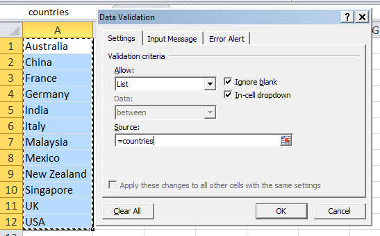
5. Pick List from the Allow: dropdown box. See screenshot above.

6. Key in the Source as =countries. This must be the name of the range you just created in Step 3. Now click OK to close this dialog box.

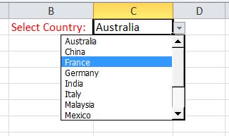
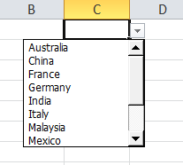
7. Once this is done, you will see a drop down arrow showing up in the cell C1. You will see the list of countries showing up here.

drop_down_filled_valuesOnce you have selected a value, it will be displayed in cell C1. No mis-spelt values. No garbage. Pure, good, data validation at its best!

You could have your master list of countries on another sheet in the same workbook, or in the same worksheet. If you do not want your users to see the individual names, you could hide the sheet and even protect it from any changes. But these things will be covered in a separate lesson.

Hope this helps. Do post a comment if you enjoy this little tip!

Cheers,
Vinai

Are you facing any problem in using Excel? Any Question?

You have come to the right place. Tell us your needs. We’ll be glad to help you!

Showing The Hidden First Column in Excel

It is quite easy to show or hide columns in Excel. Simply select a column, and press Control + 0 . The column is hidden from the view. You can make it out because of a dark line separating the columns. If you hide the B column, you will only see column A & Column C, and it is apparent that column B is hidden.

To unhide, simply select both column A & Column C. Then right click and select Unhide. Column B is brought back into view.

This works great most of the time. And it works in showing or hiding rows too.

Want to Improve Your Excel Skills?

Learn the Key Features of Excel Quickly & Easily, by Joining the
Online Training on Basic / Intermediate Excel.

To Get Most out of Excel, Learn the  Pivot Table techniques in our
Pivot Table Masterclass Training
!


But the problem arises when you want to hide the first column – Column A. Now it is difficult to select 2 adjacent columns, and you are unable to Unhide Column A.

Steps to Display the Hidden First Column (Column A) in Excel

  1. Press F5. The Go To dialog box will popup.
  2. Key in the cell A1 in Reference, and press Enter.
  3. The cursor would have moved to the cell A1, even if you can not see it. Do not worry.
  4. Now go to the Home Tab (in Excel 2007, 10 & 2013)
  5. Click on Format button – it is near the far end of the screen… toward the right side of the ribbon.
  6. Choose Visibility > Hide & Unhide. Then select to Unhide Columns.

    Unhide columns or Rows in Excel
    Unhide columns or Rows in Excel
  7. Voila! You will now be able to see the column A. It has been un-hidden.

It is a simple trick. Excel is all about simple tips and tricks… The more you practice, the more you try, the more gold shall ye find!

Cheers,
Vinai Prakash

Are you facing any problem in using Excel? Any Question?

You have come to the right place. Tell us your needs. We’ll be glad to help you!

Displaying Large Numbers in K (thousands) or M (millions) in Excel

My clients keep asking me to display large numbers like in Thousands or Million to display in a shorter form. In the business world, K or M are used to represent Thousands or Millions.

For my own small Training business, I haven’t reached the revenue target of Million Dollar Sales…

But yes, I do achieve sales of several thousand from my blogs each month (PMChamp &  ExcelChamp) and my Training company in Singapore & SkillsFuture Training Courses in Singapore.

How to Show Large numbers in K or M within Excel
Large Numbers showing in K or M in Excel

However, my clients are usually small and medium enterprises as well as Multi-national companies, whose revenue is usually in Millions and sometimes in Billions too 🙂

Difficult to Read, Large Numbers look ugly in Excel
The problem is that for some people, it becomes difficult to read numbers and figures in Thousands, Millions and Billions, with so many zeroes to count.

And for our neighbouring country Indonesia, the currency denomination is so small, that a rent of a one-room apartment in Jakarta may be anywhere from 5 million to 10 million Indonesian Rupiah. So you can easily imagine how doing a simple budgeting exercise can take you into dizzying heights of billions and trillions.

How To Add a Thousand or Million Suffix to Numbers in Excel

For huge numbers, it is easier to read $23M or $25K rather than  $23,000,000  or $23,000.

So let’s see how you can convert a large number in Thousands, Millions or Billions to be an easy to read number with Microsoft Excel.

  1. Simply select the number cell, or a range of numbers that you would like to convert into K or M.
  2. Right Click, and choose Custom Formatting.
    You can also choose Number Formatting from the Home Ribbon, or simply press the shortcut  [Ctrl] + 1.
  3. Go to Custom, and key in 0, “K” in the place where it says General. Now close the Format Cells popup window.Custom Number Format Popup in Microsoft ExcelCustom Number Format Popup in Microsoft Excel
  4.  Voila! Now your large number will be displayed in Thousands. So 23000 becomes 23K.

How To Display Numbers in Millions in Excel

  1. Right-Click any number you want to convert. Go to Format Cells. In the pop-up window, move to Custom formatting.
  2. If you want to show the numbers in Millions, simply change the format from General to 0,,”M”.  The figures will now be 23M. So essentially we are adding 2 commas instead of a single comma this time.
  3. If you would like to see the decimal point for the millions figure, like 23.6M, you can format it to 0.0,,”M”
  4. What’s great is that if you now create a chart on this data, the chart or Pivot Table will now show the figure in this custom format.
  5. Thus you will see the chart displaying numbers in Millions, or Thousands… saving space, and making the chart or pivot easier to read and analyze.

That’s it! Spend more time analyzing, not staring at the huge numbers 😉

You can check this out for yourself, by downloading the Sample Excel File. It has a few scenarios where you can try to convert large numbers into Millions or Thousands, whatever you prefer.

Sample Excel File Download: Number_formatting_in_K_or_M.xlsx

This technique applies to Excel 2003, Excel 2007, Excel 2010,  Excel 2013, Excel 2016, Excel 2019 & Microsoft Office 365 editions.

It would work in all versions of Microsoft Excel in the past 20 years…

Hope it helps! Do share it with others on Facebook or LinkedIn.

And do comment or write to tell me of any issues you are facing in using Excel every day. There may be a simple solution that can save you a lot of time. At ExcelChamp, I solve many small problems each day to make Excel easy for everyone.

Are you facing any problem in using Excel? Any Question?

You have come to the right place. Tell us your needs. We’ll be glad to help you!

Cheers
Vinai Prakash

Need Tips on Pivot Tables, Data Analysis or Creating Better Charts?

Do checkout these resources

And if you want to learn Advanced Excel fast, then check out our detailed guide. Plus Master Lookup Functions like VLOOKUP, HLOOKUP, INDEX in Excel.

Want to Improve Your Excel Skills?

Learn the Key Features of Excel Quickly & Easily, by Joining the
Online Training on Basic / Intermediate Excel.

To Get Most out of Excel, Learn the  Pivot Table techniques in our
Pivot Table Masterclass Training
!

FREE COURSE ON PIVOT TABLES TO ANALYZE DATA – Click & Start watching Videos For Free and improve your Pivot Table Skills. No signup is required.

Extracting Text From Variable Length Strings

After I wrote about how to extract characters from the left, right or middle of a text string in Excel, I received a few inquiries about extracting text from strings which don’t seem to have a fixed size, and vary in length.

For example, if the data is something like this

HQ-1022-PORT
LONDON-4053-LANDED
HOUSTON-2488-WEST
SINGAPORE-3133-LEEDON

You want to separate out the first word (HQ, LONDON, HOUSTON, SINGAPORE etc.)

Can’t Use LEFT Function
You can’t use a LEFT function, because a left function needs to know the number of characters you want to extract. And this itself is variable… There are 2 characters in HQ, 6 in London, 7 in Houston etc.

One of the ways I have discovered is to find the location of the first Hyphen (-), and extract all characters from the left of it.

Want to Improve Your Excel Skills?

Learn the Key Features of Excel Quickly & Easily, by Joining the
Online Training on Basic / Intermediate Excel.

To Get Most out of Excel, Learn the  Pivot Table techniques in our
Pivot Table Masterclass Training
!


Finding the location of the First Hyphen
We can use the FIND function to find the location of the first hyphen.

If A2 contains HQ-1022-PORT, we can use the formula as:

=FIND(“-“,A2)

The answer would be 3. This means that the hyphen is the third character in the string. This is perfect. Now we know that we need n-1, that means 3-1, which is 2. We need 2 characters from the Left of this number.

So we can write another formula as

=LEFT(A2,  FIND(“-“,A2)-1 )

The resulting answer would be HQ. Copy the formula down to other cells, and you should be able to extract HOUSTON, SINGAPORE etc. without much hassle, and without having to write another, different formula.

One size fits all formula to extract a variable length string from a piece of text. And pretty easily too!

Do you have any other method? How would you solve this challenge?

Please post your answers in the comments below.

Cheers,
Vinai Prakash

P.S. – I am teaching a 2 day course on Data Interpretation & Analysis in Singapore on Feb 9-10, 2015, and another on March 9-10, 2015. If you would like to learn techniques to analyze data and create management reports, you can attend this program.

Awaiting you and your innovative comments below … 🙂 – Vinai

Are you facing any problem in using Excel? Any Question?

You have come to the right place. Tell us your needs. We’ll be glad to help you!

Quick Tip: Re-Sorting a List or Table in Excel

Of course you know how to sort data in Excel! Simply click on the Sort button, or click on the mini A-Z or Z-A chicklet buttons, and voila! the list is sorted. And if you want more control, you can try Custom Sorting, and Advanced Sorting with this Method.

The problem is that a sorted list often gets out of sync, if you keep adding or editing data in the table. And if you use a Custom Sorting sequence, you can’t simply click on the single column sorting chicklets any longer  🙁

So you have to go to Custom Sort, and click it again to get the list sorted one more time.

Want to Improve Your Excel Skills?

Learn the Key Features of Excel Quickly & Easily, by Joining the
Online Training on Basic / Intermediate Excel.

To Get Most out of Excel, Learn the  Pivot Table techniques in our
Pivot Table Masterclass Training
!


A Quick Way to Sort Your Custom Sorted Table in Excel
Fortunately, there is a quicker and shorter way. All you need to do is to click on the Reapply button, which shows up once you click on the Sort menu on the Home Tab.

Reapply Sorting in Excel

There’s a shortcut – Ctrl + Alt + L

This makes the current list or table sorted again. Even if you had multiple columns in the custom sorted list.

What I have done is to put this Reapply button on my Quick Access Toolbar in Excel. This makes it much snappier to apply it anytime, anywhere in Excel.

Reapply Sorting Button in the Quick Access Toolbar

Hope you like this quick tip. It has saved me quite a few clicks, and a lot of time searching for something in a not so sorted table…

Cheers,
Vinai Prakash

PS: Check out how to sort in a unique manner – not ascending , not descending. Sorting it Your Way!

Also, let me know if there is anything in Excel that bothers you…. anything where you could get some help. Simply post it into a comment or email it to me, and I’ll see what I can do to help you out 🙂 – Vinai

Are you facing any problem in using Excel? Any Question?

You have come to the right place. Tell us your needs. We’ll be glad to help you!