Different Grouping For Multiple Pivot Tables Based on Same DataSet

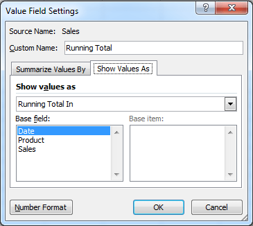
One of the key features of Pivot Tables is to summarize the information quickly. Another great advantage is its ability to look at percentages – percent of total, percent of grand total, percent of row total, running total in etc.

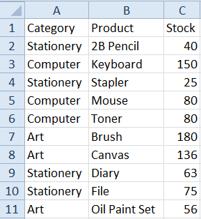
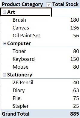
Yet another fantastic feature is the ability to group data in Excel – either by existing columns, or by creating your own custom logic. Data can be grouped by Text Columns or even Date Columns. And the result is instantly summarized. Amazing stuff!

All is good so far… The problem crops up when you have created some grouping, and then decide to build another pivot table to get another view of the same data, while keeping the original pivot table in place.

The second pivot table automatically groups the data based on the first pivot’s grouping. And if you change the grouping on the second pivot, the first pivot table changes too.. Bo hoo hoo 🙁

This can be frustrating and sometimes difficult to troubleshoot or fix.

Why does a Pivot Table share its Grouping with another Pivot Table?

That’s because both the pivot tables are sharing the same pivot cache. To understand better, when Excel creates a pivot table, it makes a copy of the entire source data, and creates a temporary pivot cache in the memory. This duplicated cache is now stored with the Excel file, doubling its size. If your source data was huge, the excel file soon soars in size too.

To save hard drive space and memory, when the second pivot table was created, it used the same cache as the first pivot table. This makes sense, but then since the cache is shared, change in the cache for one pivot table affects the other pivot table too.

The solution is to have a separate pivot cache for the second pivot table.

How to Create a Separate Cache for the Second Pivot Table?

Although this method will use up more memory, it is a good solution, works well, and hardly takes any time to implement.

Select the source data, go to the Formulas tab, and click on Define Name button.

Key in a unique name in the popup. Let’s say you call this DataSet1. This creates a Unique Named Range.

Now click on the Define Name button once more, and create another name for the same data set. Let’s call this DataSet2.

Create Pivot Tables with Unique Data Sets

Now create the first pivot table based on the first Data set (DataSet1). Group on whatever fields you want. Once you are happy with the result, do the same thing for the second pivot table.

Just remember to use the second data set for the second pivot table (DataSet2). Group the data on a different field.

Want to Improve Your Excel Skills?

Learn the Key Features of Excel Quickly & Easily, by Joining the
Online Training on Basic / Intermediate Excel.

To Get Most out of Excel, Learn the  Pivot Table techniques in our
Pivot Table Masterclass Training
!


You will notice that the grouping of the second table stays, and it does not alter the grouping order of the first pivot table. That’s because we are using different defined names.

Thus, Excel creates two different pivot caches, and even though both refer to the same data set, it is transparent to Excel, and is of no consequence.

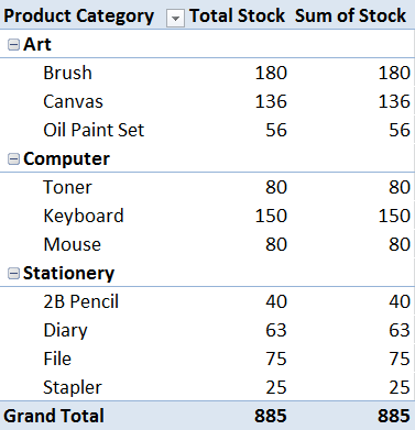
Now you can enjoy the benefits of two different views, one with one set of grouping, and another with another set of grouping.

Although this method inflates the size of the file, it is a quick and dirty method, that works well. Try it out… and let me know how it goes…

Cheers,Vinai Prakash,
Founder of ExcelChamp.Net

Additional Resources:
If you found this tip useful, you may want to subscribe to the ExcelChamp Weekly Excel Tips Newsletter.

And check out these cool Excel Tips too…

Cheers – Vinai

Are you facing any problem in using Excel? Any Question?

You have come to the right place. Tell us your needs. We’ll be glad to help you!

How To Get Running Totals In a Pivot Table

Pivot Tables are great in summarizing data from thousands of rows in just seconds. You can get Sum, Count, Average of numbers from any grouping in a Pivot table.

But the one thing that you need at times is a running total in a column. For example, in January, you sold 100 cans, and in February you sold 120 cans. So the total cans you sold till Feb is 100+120=220. This is a running total up to the month of February.

If you want Excel to do this, you can write a formula in the data cells. But to get this thing done in a Pivot Table, you need to use a different way. And it is already pre-built in  Excel Pivot Tables, starting from Microsoft Excel 1995.

Raw data for Pivot Table

All you need to do is to click on the Data Field in the Pivot Table Field List, and a popup comes up.

Choose the last option – Value Field Settings.

Move to the Second Tab – Show Values As.

Then select “Running Total in” in the drop-down. Select a base field. It must be a text field, like Product, Category, Region etc.

Show Values As - Running Total In
Show Values As – Running Total In

Voila, you get a running total in the data field inside the pivot table. And all you did was to select the correct option. No formulas to write… no calculations to make or check. Isn’t it wonderful?

Running Totals Calculated

Using % Running Total In

Similarly, if you choose % Running Total In as the calculation, the running total numbers would be displayed as a percentage of the total. Giving you a much nicer perspective.

Running total Percentage in Excel Pivot
Percentage of Running total

Want to Improve Your Excel Skills?

Learn the Key Features of Excel Quickly & Easily, by Joining the
Online Training on Basic / Intermediate Excel.

To Get Most out of Excel, Learn the  Pivot Table techniques in our
Pivot Table Masterclass Training
!


If you’d like to learn more Excel Pivot Table Tricks, here are some additional articles:

Questions About Pivot Tables in Excel?

If you have any questions regarding Pivot Tables in Excel, simply post a comment below and I’ll help you with it. All the best!

And Subscribe to our Excel Tips Newsletter, so we can send you more such Pivot Table Techniques by email. Only useful stuff, without the hype. And we won’t spam you. So don’t worry. Just subscribe.

Cheers,
Vinai Prakash
Founder of ExcelChamp.Net

Vinai conducts 1-2 day seminars and Training Sessions on Microsoft Excel all over the world, helping companies maximize their productivity in using Microsoft Excel. If you would like to find out more, simply contact us.

Are you facing any problem in using Excel? Any Question?

You have come to the right place. Tell us your needs. We’ll be glad to help you!

How To Show Values & Percentages in Excel Pivot Tables

Want to Be a Power Analyst?

They have a secret… The power analysts NEVER, repeat NEVER report any raw numbers directly.

They only talk in PERCENTAGES!

  • there were 4.3% new jobs created in the last quarter, 
  • the economy shrank 2.45% year on year…
  • the ROI increased 5.34% in this month compared to the previous month, or
  • the customer service satisfaction index improved by 4.8% this quarter, over the industry average…

This is how analysts speak. So up your game, and speak in Percentages only from now onwards…

But where do you get all these percentages from in Excel?

To create a Percentage Table in Excel, all you need to do is to learn the simple Pivot Table techniques of Excel.

These techniques help you to show both values and percentages at the same time. It’s like having your cake and eating it too!

Pivot Table Showing Values & Percentages

Ever since I published the How to Analyze data with Pivot Tables Video on YouTube, I receive an average of 2-3 new queries every day, asking for more tips on getting more juice out of using Pivot Tables in Microsoft Excel. I have now created the ultimate guide of 10 Methods to Summarize Data in Excel.

This tip about showing Percentages in the Pivot table is pretty simple, yet it could make you into the next Power Analyst you see on CNBC or other TV News channels.

You see, analysts crunch numbers on Business Shows, News Channels all day long. And they make it look so sexy, so cool….

They talk about Year or Year Growth, Quarterly Income Growths, Dividend per share, and most importantly, the presentation has an impact on you… because they talk about percentages.

Simply learn this neat trick to Display Values & Percentages in Excel Pivot Tables.

Yes, a simple “We have 528 widgets” does not make anyone notice the numbers or their impact on the business.

But the same thing converted into “28% of our inventory is stuck in widgets” can make a big difference and make people take notice of what you say.

Want to Improve Your Excel Skills?

Learn the Key Features of Excel Quickly & Easily, by Joining the
Online Training on Basic / Intermediate Excel.

To Get Most out of Excel, Learn the  Pivot Table techniques in our
Pivot Table Masterclass Training
!

How to Convert Numbers Into Percentages?

Well, most of the time, this nifty trick can be done using the basic Pivot Table in Excel. And the version of Excel does not matter. You could use Excel 2010, Excel 2013, Excel 2016, Excel 2019 or even the latest Microsoft  Office Excel 365. Pretty much any version of Excel will do.

Let’s say you are showing Categories, Products and their inventory in a Pivot Table like below.

Rawdata before Pivot Creation

It is useful to see the inventory by category, but it does not clarify things. So let’s add some clarity to our Pivot table, by adding a percentage.

Adding a Percentage Column in the Pivot Table

Inventory by Category in Pivot

If you just drag the Stock field to the Values section of the Pivot Table one more time, the output Pivot Table would look like this.

after_adding_second_value_in_pivot
Pivot Table showing 2 identical sets of columns for the values

Now you click the Second Stock Field (Sum of Stock) in the Values section and click on it again. You will see a popup like below.

Show Value As Popup in Microsoft Excel 2010
Show Value as Popup

Choose Show Value As > % of Grand Total. In some versions of Excel, it might show as % of Total. This is fine.

Newer versions of Excel,  like Excel 2016, Excel 2019 or Microsoft 365, show a % of Grand Total when you right-click on any numeric value. This is the key way to create a percentage table in Excel Pivots.

The Pivot view now changes to this:

Pivot with Values & Percentages
Pivot showing Values & Percentages both at the same time

Isn’t it magical! Now you can see that the Art category accounts for 42% Inventory, and Computer Products account for 35%, followed by Stationery, at 23%.

After converting the raw numbers into percentages, it is more insightful than looking at absolute numbers only.

And applying such nifty techniques to create a Percentage Table converts you into a Power Analyst who talks in Percentages, not just numbers.

Use this neat trick to convert numbers into percentages, and especially convert it to a % of Grant Total. It is a really useful technique.

I am sure you will love this simple technique.  Hope it helps! Do share it with others on Facebook or LinkedIn.

And do comment or write to tell me of any issues you are facing in using Excel every day. There may be a simple solution that can save you a lot of time. At ExcelChamp, I solve many small problems each day to make Excel easy for everyone.

Are you facing any problem in using Excel? Any Question?

You have come to the right place. Tell us your needs. We’ll be glad to help you!

Cheers
Vinai Prakash

Need Tips on Pivot Tables, Data Analysis or Creating Better Charts?

Do check out these useful articles & Video Resources

And if you want to learn Advanced Excel fast, then check out our detailed guide.

Want to Improve Your Excel Skills?

Learn the Key Features of Excel Quickly & Easily, by Joining the
Online Training on Basic / Intermediate Excel.

To Get Most out of Excel, Learn the  Pivot Table techniques in our
Pivot Table Masterclass Training
!

Do You Use These Features of Microsoft Excel?

Most people hardly use the most useful features available in Microsoft Excel. Many are just using Excel as a calculator to do basic calculations like adding or subtracting numbers. This is a gross under use of Excel’s vast potential and feature rich functionality.

Do a quick check, and see if you use these advanced features of Microsoft Excel in your day to day work to improve your productivity and efficiency.

  1. Finding the Top 10 Customers or Finding the Bottom 5 Performers in the organization
  2. Give Names to Range of Cells, and then use them in formulas for easy referencing and decoding – like =Salary – CPF + Allowance
  3. Exploit Pivot Tables to Summarize the data and slice & dice it in any way – like finding sales by product groups, or calculating productivity by department, or calculating sales by department by product by area.
  4. Write Macros to automate routine things that save you a huge amount of time – example creating different pivots, charts, tables, and doing complex calculations, or compiling the cost benefit ration, cash flow statement automatically.
  5. Highlight values that are above or below a certain threshold – like all sales above $25,000 to be highlighted, or all products with a net profit margin of less than 5% be highlighted.
  6. Sort the values in Ascending, Descending or any Customized sorting order – like sorting in order of Manufacturing, Accounts, Sales departments.
  7. Use advanced filtering conditions, and be able to filter data using multiple different criteria – like salary > 50,000 and sales <100,000 or Zone in East, West.
  8. Create fantastic charts that portray the given business situation perfectly. There are over 50 different types of charts to choose from, and each has its edge, advantages and a reason. Do you know when to use which type of chart – like two axis charts, stacked column and line charts, bubble charts, pie, slice of a pie etc.
  9. Create management dashboard that are dynamic, and provide a complete snapshot of the key business KPIs in the company – change the chart values at the click of a checkbox or change in a dropdown value
  10. Use Excel’s advanced What-If analysis to do projections for future, forecasting, trend analysis etc. with ease
  11. Use Lookup tables to find any value or corresponding value from a table using advanced functions and formulas – find values that in the left of the looked up value
  12. Protect certain cells from data entry, and hide the formulas from other cells. Ensure that only certain values are keyed in the cells to avoid data discrepancies.

Want to Improve Your Excel Skills?

Learn the Key Features of Excel Quickly & Easily, by Joining the
Online Training on Basic / Intermediate Excel.

To Get Most out of Excel, Learn the  Pivot Table techniques in our
Pivot Table Masterclass Training
!


This is just the tip of the iceberg… These are common things that can be done easily with Excel’s in-built features.

So how many of these did you know? And how many would you like to learn more about? Even if you learn one new trick in Excel, it will save you immense time and improve your productivity. Investing in Microsoft Excel Training bears fruit in no time, and is a no brainer.

Microsoft Excel is really extremely powerful. Each version of Microsoft Excel – be it Excel 2007, or Excel 2010 or Excel 2013, Excel 2016 or Office 365 adds more and more features to the already powerful dynamite of a package.

At ExcelChamp, we teach people how to leverage the maximum power out of Microsoft Excel in short training courses.

So what are you waiting for? If you would like to learn any one or more of such useful features of Microsoft Excel, just let us know. We provide online training through videos, which will show you each click, step by step, so you can master the new techniques easily, with exercises, and practical examples.

Go ahead, equip your team with the right skills. Get everyone on board to learn the basic and advanced features of Microsoft Excel, and Be Awesome in Excel!

Email to us to know more about Online Excel Training at ExcelChamp.Net.

Cheers,
VInai Prakash, PMP, ITIL, GAP, Six Sigma, Excel Guru

Are you facing any problem in using Excel? Any Question?

You have come to the right place. Tell us your needs. We’ll be glad to help you!

How to Analyze Data using Excel Pivot Tables

Do you know how easy it is to use the Pivot Tables in Excel, for Data Analysis?

To demonstrate this, I went to the Internet, and  found some travel data. It belongs to an unnamed Travel Company. The travel company collects the amount of ticket sales, the age of the passenger, and their gender only.

Based on this, how do we analyze the data, and find some hidden gems of information that can make the data come alive, and aid us in doing some real life Marketing.

Watch this step by step video on analyzing this data, using the Pivot Table technique in Microsoft Excel. I am using Excel 2010 version for this demonstration.

As you can see, many hidden insights can be found by using the Pivot Tables in Excel. So get started… Use them in your day to day work, and become a Data Analyst, rather than a Data Gatherer or Data Reporter…

Want to Improve Your Excel Skills?

Learn the Key Features of Excel Quickly & Easily, by Joining the
Online Training on Basic / Intermediate Excel.

To Get Most out of Excel, Learn the  Pivot Table techniques in our
Pivot Table Masterclass Training
!


Have you subscribed to the ExcelChamp.Net Email Newsletter, where we send you such tips by email?

Additional Resources

Cheers,
Vinai Prakash, PMP, ITIL, MBA, GAP
Founder: ExcelChamp.Net – Providing Everyday Tips for Improving Productivity, Using Excel!

Are you facing any problem in using Excel? Any Question?

You have come to the right place. Tell us your needs. We’ll be glad to help you!

<div class=”ml-form-embed”
data-account=”3112195:l6l5i4i1x0″
data-form=”5497493:o9q9a8″>
</div>

Additional Resources for Learning Excel & Become A Pro

  1. Top 12 Most Important Excel Functions You Absolutely Must Know
  2. Excel Beginners Guide
  3. Excel Essentials: From Beginner To Pro in Just 6 Weeks