Vinai Prakash

Vinai Prakash is the founder and master trainer of ExcelChamp.Net. Vinai has over 30 years of experience in using Excel, and is a Data Warehousing & Business Intelligence Professional. Vinai has coached and trained over 30,000 professionals in using Excel, Power BI, Python, SQL, and regularly runs Excel Data Analysis, Excel Dashboard MasterClass, Excel for Beginners, Advanced Excel MasterClass online and all over the world. Vinai's Videos on YouTube channel and his blog articles and newsletters are read by thousands of subscribers all over the world. Vinai lives in Singapore with his wife and 2 kids.

Multiple Ways to Count in Excel

December 3, 2023August 3, 2014 by Vinai Prakash

Counting the number of cells containing values, counting number of cells meeting a certain criteria, counting names, counting cells in a range…. you name it, there is a need to count in Excel. And there are multiple ways to count in Excel. Some techniques are more helpful than others, and some can provide unique insights which others can’t produce.

Let’s look at the different ways to count in Excel, and their relative benefits.

1. Count the number of cells with values: The simplest way is to use the inbuilt function Count. Select the cell range, and out comes the cou nt of cells in the range.

Count only works with counting of Numeric information. If you try to count names, you will get a ZERO.

To count alphanumeric values – values with names, categories, text, serial numbers etc., then you must use the variation of Count – called COUNTA. This function is to count Alphanumeric data.

Count of Numbers in a Range, & Count of Names in a Range

2. Using a Criteria to Count specific Cells: There are several ways to count the cells that meet a certain criteria. The first method treats the data as a database, and uses the Database Functions within Excel.

=DCOUNT(Database, Field, Criteria)

Count the cells that meet a specific criteria using Dcount

Here A4:C12 is the entire data, B4 is the cell column that we want to count, and the criteria is Age should be greater than 30 years (B1:B2) cells.

The answer for this count is 5. See if you got this correct.

The database functions have been existing in Excel since 1995. They treated Excel data as a database like Oracle, Dbase etc. These database functions DSUM, DCOUNT, DAVERAGE etc. are quite useful, and are available for backward compatibility, although the same work can be accomplished by other functions equally well too.

3. Using COUNTIF Function to count cell conditionally. This method evaluates the cells against the condition, and if it matches, it is counted.

=COUNTIF(Cells, criteria)

Here, the cells that contain the data is provided first, and the second argument is the criteria. The headings are not really needed. Each cell in the first range is checked against the criteria, and if the criteria matches, the record is counted, otherwise it is ignored.

And if you have multiple criteria to check for, you can use the COUNTIFS which can take multiple criteria arguments.

CountIFS to count cells with multiple criteria cells.

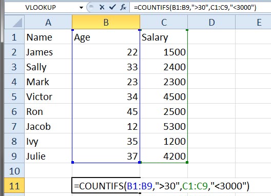
The formula in the picture captures the count of cells that are having age of >30years, and Salary less than $3000. Answer is 3.

So as you can see, there are multiple functions, and ways to count cells in Excel. It depends on whether you want to count numbers or textual data. It also depends if you have conditions or not.

Use these functions to count in multiple ways… Happy counting!

Cheers
Vinai Prakash

Are you facing any problem in using Excel? Any Question?

You have come to the right place. Tell us your needs. We’ll be glad to help you!

Additional Resources for Learning Excel & Become A Pro

Creating Beautiful Excel Charts For Business Presentations

July 11, 2022August 2, 2014 by Vinai Prakash

Microsoft Excel is used to produce charts that are used in the boardroom, in business presentation, and in school projects all over the world. However, most people do not go beyond the standard charts that Excel produces by default, which could be the most boring, and most unsuitable of charts.

In this article, I am going to show you how you can add value to the default Excel chart, and make it really sing, with just a few clicks. Plus a few tips on how to put some glamor, some jazz, some oomph to your charts to make them beautiful, sexy and cool!

Remove Chart Junk: The default Excel chart has a lot of junk. See the before and after picture below.

Now let’s see how to arrive at this result ourselves. If you would like to try it yourself, see the image above for the Excel data file with the original data showing. You can key in this data to get started yourself.

1. Move Legend to the Bottom: The default Legend on the right side of the chart steals away valuable space from the chart. So move it to the bottom. Simply Go to Chart Layout Settings, and Click Legend, then select Bottom. The legend moves to the bottom, and the chart bars now have more space to expand.

2. Remove Grid Lines: Sometimes the grid lines do not add much value, and are best eliminated, as they just make the graph look cluttered.

3. Show Data Values: You can show data values on top of the bars, inside the bars, or at the bottom. Once you have the data bars showing, you really do not need the grid lines anyway.

4. Remove the Vertical Axis: If the values of the data bars, and the Title of the chart are self explanatory, then you can get rid of the vertical axis, giving you more room.

5. Add a Chart Title, Above the Chart: Choose the Title from the Layout, and then select “Above Chart”. This way, your data will never hit the title.

6. Change the Theme: Most people live the default Office theme. But Excel provides over 50 different themes, which can make your charts look much sharper, out of the box.

7. Apply Custom Colours: If the theme colours do not suit you, you can pick any colour you like for any data bar or pie.

8. Add a Company Logo: You can add an image anywhere in the chart. It could be your company logo, or any particular product. Do not add clipart for the sake of adding it. It looks quite cheap and amateurish.

With these simple tips, you can improve your charts and graphs, and give them a new lease of life… make ’em jazzy, snappy, and cool!

Cheers,
Vinai Prakash

Are you facing any problem in using Excel? Any Question?

You have come to the right place. Tell us your needs. We’ll be glad to help you!

Top 10 Time Saving Tips in Using Microsoft Excel

December 3, 2023February 10, 2014 by Vinai Prakash

If you are a data warrior, chances are that you use Excel extensively in your day to day work. Learn to Analyze Data Quickly With Excel.

And there are many ways to boost productivity within Excel. Use these nifty tricks and improve productivity.

1. View All Formulas in Excel With a Single Click: I wrote about this trick some time back. It allows you to view all the formula with a single click of Control + ` Key. This acts like a toggle key. This can save a lot of time in finding where are the formulas to edit/view them.

2. Clean up Your Data – Identify the Duplicates, and Remove Duplicates: There is no point in having duplicates in your tables. There are multiple ways to do this. You can identify the duplicates, and then choose to remove them manually, or you can request Excel to remove the duplicate rows completely, automatically.

3. Colour Alternate Rows and Make it Easier to Read Large Data Sets: Prior to Excel 2007, we used to write formulas to colour alternate rows in Excel. This makes it easier to read the data.

=MOD(ROW(),2)=0

This function would tell us if the row is an even row or an odd row, and then we could colour it.

But since Excel 2007, we can do this in multiple ways. We can convert the data into a table. And in the table options, you can then colour alternate rows or columns as bands.

And then you can also use the formula above, and use conditional formatting.

4. Learn The In-Built Functions in Excel: Many people are amazed at the plethora of in-built functions available in Excel. But you must know that they exist, and also know the syntax to make a good use of them.

5. Learn and Use Pivot Tables Effectively: Pivot tables summarize data quickly. Learn to use them effectively. Simple techniques like displaying both values and percentages in a Pivot Table adds extra value.

Similarly, learn to show different grouping for different pivot tables, even though it is based on the same data source. Also, creating a calculated field in a pivot table adds extra value.

If you are new to pivot tables, this introduction on how to analyze data using Excel pivots will be useful.

6. Charting Techniques Can Make People Notice Your Work: Creating nifty charts like the 2 Axis chart, or the PivotChart can be useful in the board room. Learn these techniques. Similarly, using Slicers in Pivot Charts can make dynamic Charts that can wow the audience. They are simple to use.

7. Get Back to Your Selection: Many times you will select or highlight some cells, but then move about the Excel file to find something. Then your are lost. Now you don’t remember where exactly is your selection. Simply click Control + Backspace. It will take you to the highlighted area in a blink!

8. Use Range Names to Refer to Cells: Instead of using G3, C3 or F3, you can give each cell a name. Not only single cells, you can actually define a name for a group of cells too. Then you can refer this group of cells by a particular name.

So instead of saying =G3+C3-F3, you can now calculate Salary as

=Basic_Pay + Allowance – Tax

This is much easier to read, and comprehend. No need to look up where the formulas are coming from, as the names are self evident.

9. Learn Excel Shortcuts: There are hundreds of shortcut combinations in Excel. It is impossible to remember all of them. But you must know a few to really speed up your work. Some of my favorites are:

Control N: New workbook
Control `: View All Formulas
Control Backspace: Jump to selected Cells
Alt + F1: Creates a inserts a chart based on the currently selected data as an embedded chart object.
Alt + =: Auto sum formula is inserted
Ctrl + Shift + Enter: Enter an Array Formula
F9: Calculates all the worksheets in all open workbooks

See More of Such useful Excel Shortcut gems.

10. Learn to Use Dates Effectively: In Excel, dates are stored as numbers. They can be displayed in a wide variety of Formats. Understand these formats to display them in the way that suits the applications.

Also, you can calculate using dates, for example, you can find the difference between any two dates. You can add a fixed number of days to a date.

Hope you enjoyed these tips, and will use them to improve your productivity in using Excel. Do post a comment below to talk about your favorite tips in Excel.

If you wish, you can get a good book on Excel from the Excel BookStore. These books are usually quite inexpensive, and will give you many ideas to improve too.

Cheers,
Vinai Prakash, PMP, MBA, ITIL, GAP, Six Sigma

Are you facing any problem in using Excel? Any Question?

You have come to the right place. Tell us your needs. We’ll be glad to help you!

P.S. : You can contact us to conduct a workshop on Excel Tips and Tricks at your office.

And I hope you subscribed to the ExcelChamp Excel Tips Newsletter already. 🙂

Additional Resources for Learning Excel & Become A Pro

Creating a New Calculation in an Excel Pivot Table

July 11, 2022February 8, 2014 by Vinai Prakash

Ever since I published the article on how to display both values and percentages in a pivot table & How to Get Running Totals in Pivot Tables, I am getting more and more emails asking about the other features and tricks within Pivot Tables in Microsoft Excel.

One such useful feature is the ability to add a new calculated field, which is not even present in the base data set, but can be derived from the existing fields.

We can call such a field as Adding a New Calculated Field in the Pivot Table. Once added, it is available to you in a pivot table as a regular field, and can be summed, counted, averaged, etc. with ease.

To Add a Calculated Field, go to the Pivot Table Options Menu, and Find the “Fields, Items & Sets” drop down menu in the ribbon.

Calculated Field Menu in Excel 2010, Excel 2013

Click and select the Calculated Field from the drop down menu.

Type a field name in the Name: field.

We will key in the formula in the next blank cell. Do note that Excel already provides you with a Zero there. You need to remove the Zero first. And then begin to type your formula.

All the existing Fields are listed in the Field List below the formula.

Let’s say we have to calculate Bonus, which is 10% of the Sales Commission.

So the field Name we would give would be called Bonus.

The Formula would be =Sales Comm * 0.10

Click OK to close this popup menu.

You will now notice that a new field called Bonus is active in the Field List.

Double Click or Drag it to the Values Section of the Pivot Table Layout.

Voila! You have now created an new calculation called Bonus, based on existing values within the Pivot table, and it is now available for analysis in the Pivot Table.

You can use this simple technique to create as many pivot table fields, and enhance your analysis.

If you would like more such tips, you may subscribe to the ExcelChamp Excel Tips Newsletter or Excel Tips RSS Feed.

Cheers,
Vinai Prakash

Are you facing any problem in using Excel? Any Question?

You have come to the right place. Tell us your needs. We’ll be glad to help you!

PS: If you liked the tip, please do Like us, Stumble Upon on the Left Socials Bar, or Digg it!

Different Grouping For Multiple Pivot Tables Based on Same DataSet

July 11, 2022February 6, 2014 by Vinai Prakash

One of the key features of Pivot Tables is to summarize the information quickly. Another great advantage is its ability to look at percentages – percent of total, percent of grand total, percent of row total, running total in etc.

Yet another fantastic feature is the ability to group data in Excel – either by existing columns, or by creating your own custom logic. Data can be grouped by Text Columns or even Date Columns. And the result is instantly summarized. Amazing stuff!

All is good so far… The problem crops up when you have created some grouping, and then decide to build another pivot table to get another view of the same data, while keeping the original pivot table in place.

The second pivot table automatically groups the data based on the first pivot’s grouping. And if you change the grouping on the second pivot, the first pivot table changes too.. Bo hoo hoo 🙁

This can be frustrating and sometimes difficult to troubleshoot or fix.

Why does a Pivot Table share its Grouping with another Pivot Table?

That’s because both the pivot tables are sharing the same pivot cache. To understand better, when Excel creates a pivot table, it makes a copy of the entire source data, and creates a temporary pivot cache in the memory. This duplicated cache is now stored with the Excel file, doubling its size. If your source data was huge, the excel file soon soars in size too.

To save hard drive space and memory, when the second pivot table was created, it used the same cache as the first pivot table. This makes sense, but then since the cache is shared, change in the cache for one pivot table affects the other pivot table too.

The solution is to have a separate pivot cache for the second pivot table.

How to Create a Separate Cache for the Second Pivot Table?

Although this method will use up more memory, it is a good solution, works well, and hardly takes any time to implement.

Select the source data, go to the Formulas tab, and click on Define Name button.

Key in a unique name in the popup. Let’s say you call this DataSet1. This creates a Unique Named Range.

Now click on the Define Name button once more, and create another name for the same data set. Let’s call this DataSet2.

Create Pivot Tables with Unique Data Sets

Now create the first pivot table based on the first Data set (DataSet1). Group on whatever fields you want. Once you are happy with the result, do the same thing for the second pivot table.

Just remember to use the second data set for the second pivot table (DataSet2). Group the data on a different field.

You will notice that the grouping of the second table stays, and it does not alter the grouping order of the first pivot table. That’s because we are using different defined names.

Thus, Excel creates two different pivot caches, and even though both refer to the same data set, it is transparent to Excel, and is of no consequence.

Now you can enjoy the benefits of two different views, one with one set of grouping, and another with another set of grouping.

Although this method inflates the size of the file, it is a quick and dirty method, that works well. Try it out… and let me know how it goes…

Cheers,Vinai Prakash,
Founder of ExcelChamp.Net

Additional Resources:
If you found this tip useful, you may want to subscribe to the ExcelChamp Weekly Excel Tips Newsletter.

And check out these cool Excel Tips too…

Cheers – Vinai

Are you facing any problem in using Excel? Any Question?

You have come to the right place. Tell us your needs. We’ll be glad to help you!